Backpropagation is the foundation of the deep neural network. Usually, we consider it to be kind of ‘dark magic’ we are not able to understand. However, it should not be the black box which we stay away. In this article, I will try to explain backpropagation as well as the whole neural network step by step in the original mathematical way.
Outline
- Overview of the architecture
- Initialize parameters
- Implement forward propagation
- Compute Loss
- Implement Backward propagation
- Update parameters
1. The architecture
This neural network I’m going to explain is a 2-Layer neural network. The first layer is Linear + Sigmoid, and the second Layer is Linear + Softmax.
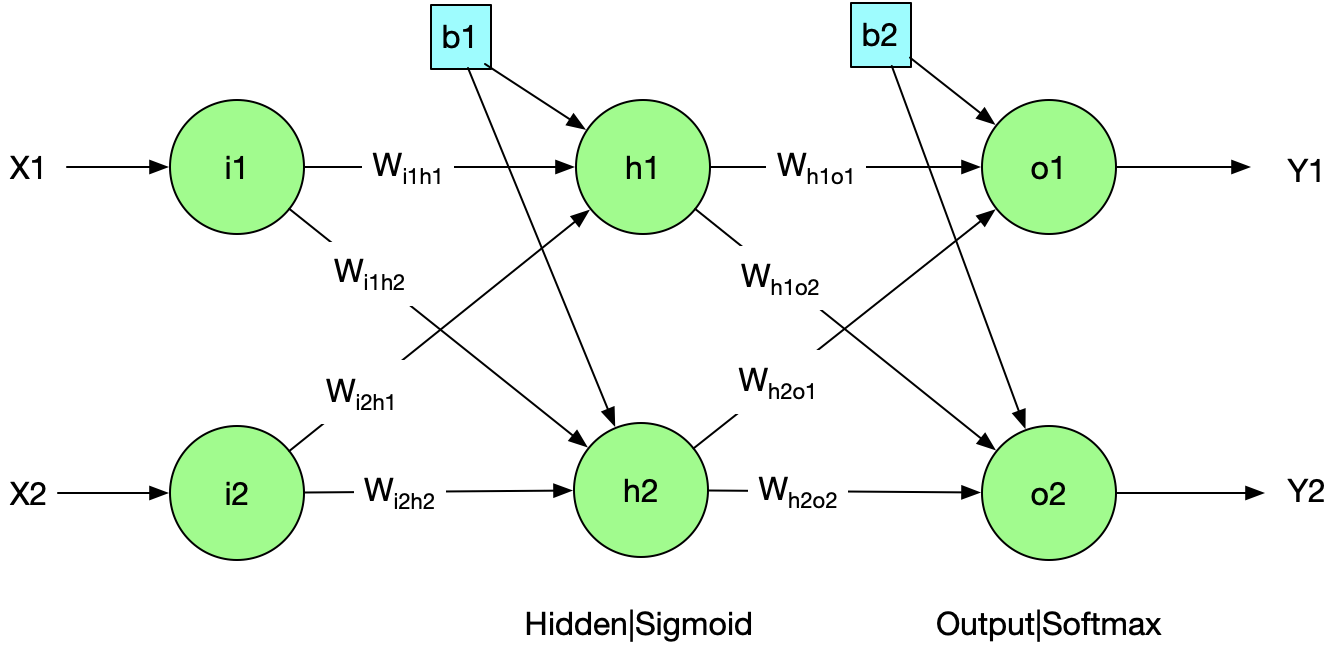
The architecture in the math formula $$ f(X)= Relu( Sigmoid( X \times W_{ih} +b_{1}) \times W_{ho} + b_{2}) $$
##2.Initialize parameters
We take one example which has two features like below $$ X= [x1, x2]= [0.1, 0.2] $$ The parameters are taken randomly. $$ W_{is}=
\begin{bmatrix} W_{i1h1} & W_{i1h2}\ W_{i2h1} & W_{i2h2} \end{bmatrix}
\begin{bmatrix} 0.7 & 0.6\ 0.5 & 0.4 \end{bmatrix} $$
$$ W_{sr}= \begin{bmatrix} W_{h1o1}&W_{h1o2}\ W_{h2o1}&W_{h2o2} \end{bmatrix}
\begin{bmatrix} 0.4&0.6\ 0.9&0.8 \end{bmatrix} $$
$$ b_{1}=[b_{11}, b_{12}] =[0.5,0.6] $$
$$ b_{2}= [b_{21}, b_{22}] = [0.7, 0.9] $$
3. Forward Propagation
3.1 Layer1:
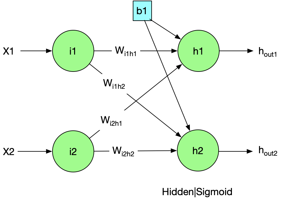
Linear
$$ X \times W_{ih} + b_{1}
[x1, x2] \times \begin{bmatrix} W_{i1h1} & W_{i1h2}\ W_{i2h1} & W_{i2h2} \end{bmatrix} + [b_{11}, b_{12}]
[0.1, 0.2] \times \begin{bmatrix} 0.7 & 0.6\ 0.5 & 0.4 \end{bmatrix} + [0.5, 0.6]
[0.67, 0.74] $$
Sigmoid
$$ Sigmoid(x)=1/(1+e^{-x}) $$
$$ [h_{out1},h_{out2}]
Sigmoid(X \times W_{ih} + b_{1}) = [Sigmoid(0.67),Sigmoid(0.74)]
[0.6615,0.6770] $$
3.2 Layer2:
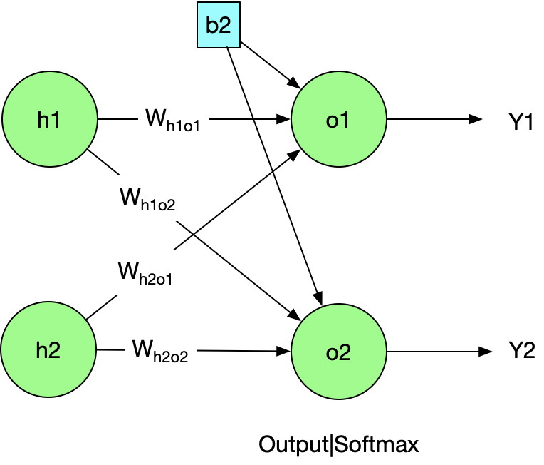
Linear
$$ [o_{in1}, o_{in2}]
[h_{out1}, h_{out2}] \times W_{ho} + b_{2}
[h_{out1}, h_{out2}] \times \begin{bmatrix} W_{h1o1} & W_{h1o2}\ W_{h2o1} & W_{h2o2} \end{bmatrix} + [b_{21}, b_{22}] =\ [0.6615, 0.6770] \times \begin{bmatrix} 0.7 & 0.5\ 0.6 & 0.4 \end{bmatrix} + [0.5, 0.6]
[1.3693, 1.0391] $$
Softmax
$$ Softmax(x){j}= \frac{e^{xj}}{\sum{i=1}^n e^{xi}} (j=1,2…n) $$
$$ [o_{out1},o_{out2}]
Softmax(X\times W_{ho} + b_{2})= [ \frac{e^{1.3693}}{e^{1.3693} +e^{1.0391}} , \frac{e^{1.0391}}{e^{1.3693} +e^{1.0391}} ]
[0.5818,0.4182] $$
##4. Compute Loss
The Loss function here we use is cross-entropy cost $$ Crossentropy= -\frac{1}{m} \sum\limits_{i = 1}^{m} (y^{(i)}\log\left(a^{[L] (i)}\right) + (1-y^{(i)})\log\left(1- a^{L}\right)) $$ The actual output should be $$ [y_{1},y_{2}]
[1.00, 0.00] $$ Since we only have one example, that means ’m = 1’, the total loss is computed as follows : $$ -\frac{1}{1} \sum\limits_{i = 1}^{1} (y_{1}\log\left(o_{out1}\right) + 0 +0 + 1log(1-o_{out2}))= -(1log(0.5818)+0+0+1*log(1-0.4182))==0.4704 $$
5. Backward Propagation
In this section, we will go through backward propagation stage by stage.
5.1 Basic Derivatives
####Sigmoid:
$$ \frac{\partial Sigmoid(x)}{\partial x}
\frac{\partial \frac{1}{(1+e^{-x})}}{\partial x}
\frac{ e^{-x}}{(1+e^{-x})^2}
(\frac{1+e^{-x}-1}{1+e^{-x}})\frac{1}{1+e^{-x}}
(1 - Sigmoid(x))\times Sigmoid(x) $$
####Softmax:
At first we know:
For $$ f(x)=\frac{g(x)}{h(x)} $$
$$ f’(x) = \frac{g’(x)h(x)-g(x)h’(x)}{[h(x)]^2} $$
Then the derivation of Softmax is $$ \frac{\partial Softmax(x)}{\partial x1}=\frac{e^{x1}(e^{x1}+e^{x2})-e^{x1}e^{x1} }{(e^{x1}+e^{x2})^2} = \frac{e^{x1+x2}}{(e^{x1}+e^{x2})^2} $$
###5.2 The backward Pass
5.2.1 Layer1-Layer2
####Weight derivatives with respect to the error
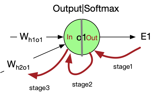
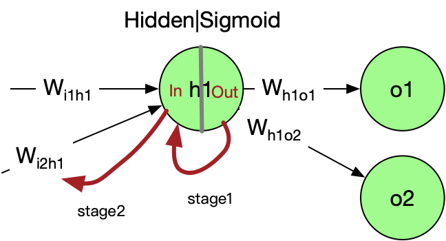
Consider Who , we want to know how Who will affect the total error, aka the value of $$ \frac{\partial E_{total}}{\partial W_{ho}} $$ Chain Rule states that: $$ \frac{\partial z}{\partial x} = \frac{\partial z}{\partial y}\cdot\frac{\partial y}{\partial x} $$ So we have $$ \frac{\partial E_{total}}{\partial W_{h2o1}}= \frac{\partial E_{total}}{\partial o_{out1}} \cdot \frac{\partial o_{out1}}{\partial o_{int1}} \cdot \frac{\partial o_{int1}}{\partial W_{h2o1}} $$ Let’s break this through stage by stage
- Stage1
$$ \frac{\partial E_{total}}{\partial o_{out1}} = \frac{\partial (-(y_{1}*log(o_{out1})+(1-y_{1})*log(1-o_{out1})))}{\partial o_{out1}}+0 =-\frac{1}{o_{out1}}=-1/0.5818=-1.719 $$
- Stage2
$$ \frac{\partial o_{1}}{\partial i_{1}}= \frac{\partial Softmax(i_{1})}{\partial i_{1}}
\frac{e^{i_{1}} e^{i_{2}}}{(e^{i_{1}}+e^{i_{2}})^2}
\frac{e^{i_{1}} e^{i_{2}}}{(e^{i_{1}}+e^{i_{2}})^2}
\frac{e^{1.3693}\cdot e^{1.0391}}{(e^{1.3693}+e^{1.0391})^2}=0.2433 $$
- Stage3
$$ \frac{\partial o_{in1}}{\partial W_{h2o1}} = \frac{\partial (h_{out1}*W_{h1o1} + h_{out2}*W_{h2o1}+b_{21})}{\partial W_{h2o1}} = h_{out2}=0.6770 $$
Finally we apply the chain rule: $$ \frac{\partial E_{total}}{\partial W_{h2o1}}= -1.719 * 0.2433 * 0.677 = -0.2831 $$ Let’s go through all the weights in Layer2 $$ W_{ho}’= \begin{bmatrix} W_{h1o1}’ & W_{h1o2}’\ W_{h2o1}’ & W_{h2o2}’ \end{bmatrix}
\begin{bmatrix} \frac{\partial E_{total}}{\partial W_{h1o1}} & \frac{\partial E_{total}}{\partial W_{h1o2}} \ \frac{\partial E_{total}}{\partial W_{h2o1}} & \frac{\partial E_{total}}{\partial W_{h2o2}} \end{bmatrix}
\begin{bmatrix} \frac{\partial E_{total}}{\partial o_{out1}} \cdot \frac{\partial o_{out1}}{\partial o_{in1}} \cdot \frac{\partial o_{in1}}{\partial W_{h1o1}} & \frac{\partial E_{total}}{\partial o_{out2}} \cdot \frac{\partial o_{out2}}{\partial o_{in2}} \cdot \frac{\partial o_{in2}}{\partial W_{h1o2}} \ \frac{\partial E_{total}}{\partial o_{out1}} \cdot \frac{\partial o_{out1}}{\partial o_{in1}} \cdot \frac{\partial o_{in1}}{\partial W_{h2o1}} & \frac{\partial E_{total}}{\partial o_{out2}} \cdot \frac{\partial o_{out2}}{\partial o_{in2}} \cdot \frac{\partial o_{in2}}{\partial W_{h2o2}} \end{bmatrix} \
\begin{bmatrix} -1.7190.24330.6615 & -2.39120.24330.6615 \ -1.7190.24330.6770 & -2.39120.24330.6770 \end{bmatrix}
\begin{bmatrix} -0.2767 & -0.3733\ -0.2831 & -0.3853 \end{bmatrix} $$
Update weights according to learning rate
Our training target is to make the prediction value approximate the correct value, while it can be transferred to minimize the error by updating weights with the help of learning rate. Suppose the learning rate is 0.02.
We got the updated weight matrix as folows $$ W_{ho}^* = \begin{bmatrix} W_{h1o1} - \eta W_{h1o1}’ & W_{h1o2} - \eta W_{h1o2}’\ W_{h2o1} - \eta W_{h2o1}’ & W_{h2o2} - \eta W_{h2o2}' \end{bmatrix}
\begin{bmatrix} 0.4 - 0.02*(-0.2767)&0.6 - 0.02*(-0.3733)\ 0.9 - 0.02*(-0.2831)&0.8 - 0.02*(-0.3853) \end{bmatrix}\
\begin{bmatrix} 0.4055 & 0.6075\ 0.9057 & 0.8077 \end{bmatrix} $$ That is the updated weight of Layer1-Layer2. The update of Input-Layer weights is the same story I will illustrate as follows.
####5.2.2 Layer0(Input Layer) - Layer1
Follow the path of the previous chapter
- Stage1:
$$ \frac{\partial h_{out1}}{\partial h_{in1}}
\frac{\partial Sigmoid(h_{in1})}{\partial h_{in1}}
Sigmoid(h_{in1})(1-Sigmoid(h_{in1})) =\ Sigmoid(0.67)(1-Sigmoid(0.67))=0.2239 $$
- Stage2:
$$ \frac{\partial h_{in1}}{\partial W_{i2h1}}
\frac{\partial(x1 * W_{i1h1} + x2 * W_{i2h1} + b11)}{\partial W_{i2h1}}
x2=0.2 $$
Apply the chain rule: $$ \frac{\partial E_{total}}{\partial W_{i2h1}}= \frac{\partial E_{total}}{\partial h_{out1}} \cdot \frac{\partial h_{out1}}{\partial h_{in1}} \cdot \frac{\partial h_{in1}}{\partial W_{i2h1}} $$ We already got the second and third derivations, regarding the first derivation, we apply the chain rule again, but in the opposite direction. $$ \frac{\partial E_{total}}{\partial h_{out1}}
\frac{\partial E_{total}}{\partial o_{out1}} \frac{\partial o_{out1}}{\partial o_{in1}} \frac{\partial o_{in1}}{\partial h1_{out}} $$ We have computed the first and second results, and the third one is merely a deviation of the linear function $$ \frac{\partial E_{total}}{\partial h_{out1}}
-1.7190.2433 \frac{\partial(h_{out1}W_{h1o1} + h_{out2}W_{h2o1})}{\partial h_{out1}} =\ -1.7190.2433W_{h1o1} =-1.7190.24330.4 =-0.1673 $$ Then we got $$ \frac{\partial E_{total}}{\partial W_{i2h1}}= -0.1673*0.2239 * 0.2=-0.0075 $$ Similarly , we can get the Layer0-Layer1 derivatives with respective to the total error $$ W_{ih}'
\begin{bmatrix} \frac{\partial E_{total}}{\partial W_{i1h1}} & \frac{\partial E_{total}}{\partial W_{i1h2}}\ \frac{\partial E_{total}}{\partial W_{i2h1}} & \frac{\partial E_{total}}{\partial W_{i2h2}} \end{bmatrix}
\begin{bmatrix} \frac{\partial E_{total}}{\partial h_{out1}} \cdot \frac{\partial h1_{out}}{\partial h1_{in}} \cdot \frac{\partial h1_{in}}{\partial W_{i1h1}} & \frac{\partial E_{total}}{\partial h_{out2}} \cdot \frac{\partial h2_{out}}{\partial h2_{in}} \cdot \frac{\partial h2_{in}}{\partial W_{i1h2}} \ \frac{\partial E_{total}}{\partial h_{out1}} \cdot \frac{\partial h_{out1}}{\partial h_{in1}} \cdot \frac{\partial h_{in1}}{\partial W_{i2h1}} & \frac{\partial E_{total}}{\partial h_{out2}} \cdot \frac{\partial h_{out2}}{\partial h_{in2}} \cdot \frac{\partial h_{in2}}{\partial W_{i2h2}} \end{bmatrix} \
\begin{bmatrix} -0.16730.2239 * 0.1 & -0.46540.21870.1\ -0.16730.2239 * 0.2 & -0.46540.21870.2 \end{bmatrix} \
\begin{bmatrix} -0.0037 & -0.0102\ -0.0075 & -0.0204 \end{bmatrix} $$
Update weights according to learning rate
Update the weights with learning rate 0.02,we got the final weight matrix $$ W_{ih}^*= \begin{bmatrix} W_{i1h1} - \eta (W_{i1h1}’) & W_{i1h2} - \eta (W_{i1h2}’)\ W_{i2h1} - \eta (W_{i2h1}’) & W_{i2h2} - \eta (W_{i2h2}’) \end{bmatrix}
\begin{bmatrix} (0.7 -0.2*(-0.0037))& (0.6 - 0.2 (-0.0102)) \ (0.5 - 0.2(-0.0075)) & (0.4 - 0.2 * (-0.0204)) \end{bmatrix} \
\begin{bmatrix} 0.7007 & 0.6020\ 0.5015 & 0.4041 \end{bmatrix} $$
###5.3 Wrap up
Finally we get all the weights updated $$ W_{ho}^* = \begin{bmatrix} 0.4055 & 0.6075\ 0.9057 & 0.8077 \end{bmatrix} $$
$$ W_{ih}^*= \begin{bmatrix} 0.7007 & 0.6020\ 0.5015 & 0.4041 \end{bmatrix} $$
6. Conclusion
- Backpropagation is beautiful designed architecture. Every gate in the diagram gets some input and makes some output, the gradients of input concerning the output indicates how strongly the gate wants the output to increase or decrease. The communication between these “smart” gates make it possible for complicated prediction or classification tasks.
- The activation function matters. Take Sigmoid as an example, and we saw the gradients of its gates “vanish” significantly to 0.00XXX, this will make the rest of backward pass almost to zero due to the multiplication in chain rule. So we should always be nervous in Sigmoid, Relu is possibly a better choice.
- If we look back to the computing process, a lot can be done when we implement the neural network with codes, such as the caching of gradients when we do forward propagation and the extracting of common gradient computation functions.
7. Reference
- https://medium.com/@14prakash/back-propagation-is-very-simple-who-made-it-complicated-97b794c97e5c.
- https://mattmazur.com/2015/03/17/a-step-by-step-backpropagation-example/.
- https://medium.com/@karpathy/yes-you-should-understand-backprop-e2f06eab496b
- http://cs231n.github.io/optimization-2/ I
- https://google-developers.appspot.com/machine-learning/crash-course/backprop-scroll/
- https://github.com/Kulbear/deep-learning-coursera/blob/master/Neural%20Networks%20and%20Deep%20Learning/Building%20your%20Deep%20Neural%20Network%20-%20Step%20by%20Step.ipynb